Neuron Segmentation¶

This tutorial provides step-by-step guidance for neuron segmentation with SENMI3D benchmark datasets. Dense neuron segmentation in electronic microscopy (EM) images belongs to the category of instance segmentation. The methodology is to first predict the affinity map (the connectivity of each pixel to neighboring pixels) with an encoder-decoder ConvNets and then generate the segmentation map using a standard segmentation algorithm (e.g., watershed).

The evaluation of segmentation results is based on the Rand Index and Variation of Information.

Tip

Before running neuron segmentation, please take a look at the notebooks to get familiar with the datasets and available utility functions in this package.

The main script to run the training and inference is pytorch_connectomics/scripts/main.py. The pytorch target affinity generation is connectomics.data.dataset.VolumeDataset.

Neighboring affinity learning¶

The affinity value between two neighboring pixels (voxels) is 1 if they belong to the same instance and 0 if they belong to different instances or at least one of them is a background pixel (voxel). An affinity map can be regarded as a more informative version of boundary map as it contains the affinity to two directions in 2D inputs and three directions (z, y and x axes) in 3D inputs.

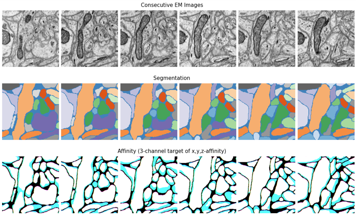
The figure above shows examples of EM images, segmentation and affinity map from the SNEMI3D dataset. Since the 3D affinity map has 3 channels, we can visualize them as RGB images.

1 - Get the data¶

wget http://rhoana.rc.fas.harvard.edu/dataset/snemi.zip

For description of the SNEMI dataset please check this page.

Note

Since for a region with dense masks, most affinity values are 1, in practice, we usually widen the instance border (erode the instance mask) to deal with the class imbalance problem and let the model make more conservative predictions to prevent merge error. This is done by setting MODEL.LABEL_EROSION = 1.

2 - Run training¶

Provide the yaml configuration files to run training:

CUDA_VISIBLE_DEVICES=0,1,2,3,4,5,6,7 python -m torch.distributed.launch \
--nproc_per_node=2 --master_port=1234 scripts/main.py --distributed \
--config-base configs/SNEMI/SNEMI-Base.yaml \
--config-file configs/SNEMI/SNEMI-Affinity-UNet.yaml

The configuration files for training can be found in configs/SNEMI/. We usually create a datasets/ folder under pytorch_connectomics and put the SNEMI dataset there. Please modify the following options according to your system configuration and data storage:

IMAGE_NAME: name of the 3D image file (HDF5 or TIFF)
LABEL_NAME: name of the 3D label file (HDF5 or TIFF)
INPUT_PATH: directory path to both input files above
OUTPUT_PATH: path to save outputs (checkpoints and Tensorboard events)
NUM_GPUS: number of GPUs
NUM_CPUS: number of CPU cores (for data loading)

Tip

By default, we use multi-process distributed training with one GPU per process (and multiple CPUs for data loading). The model is wrapped with DistributedDataParallel (DDP). For more benefits of DDP, check this tutorial. Please note that official synchronized batch normalization (SyncBN) in PyTorch is only supported with DDP.

We also support data parallel (DP) training. If the training command above does not work for your system, please use:

CUDA_VISIBLE_DEVICES=0,1,2,3,4,5,6,7 python -u scripts/main.py \
--config-base configs/SNEMI/SNEMI-Base.yaml \
--config-file configs/SNEMI/SNEMI-Affinity-UNet.yaml

DDP training is our default settings because features like automatic mixed-precision training and synchronized batch normalization are better supported for DDP. Besides, DP usually has an imbalanced GPU memory usage.

3 - Run training with pretrained model (optional)¶

(Optional) To run training starting from pretrained weights, add a checkpoint file:

CUDA_VISIBLE_DEVICES=0,1,2,3,4,5,6,7 python -m torch.distributed.launch \
--nproc_per_node=2 --master_port=1234 scripts/main.py --distributed \
--config-base configs/SNEMI/SNEMI-Base.yaml \
--config-file configs/SNEMI/SNEMI-Affinity-UNet.yaml \
--checkpoint /path/to/checkpoint/checkpoint_xxxxx.pth.tar

4 - Visualize the training progress¶

We use Tensorboard to visualize the training process. Specify --logdir with your own experiment directory, which can be different from the default one.

tensorboard --logdir outputs/SNEMI_UNet/

5 - Inference of affinity map¶

Run inference on image volumes (add --inference). During inference the model can use larger batch sizes or take bigger inputs. Test-time augmentation is also applied by default. We do not use distributed data-parallel during inference as the back-propagation is not needed.

python -u scripts/main.py --config-base configs/SNEMI/SNEMI-Base.yaml \
--config-file configs/SNEMI/SNEMI-Affinity-UNet.yaml --inference \
--checkpoint outputs/SNEMI_UNet/checkpoint_100000.pth

6 - Get segmentation¶

The last step is to generate segmentation (with external post processing packages) and run evaluation. First download the waterz package:

git clone git@github.com:zudi-lin/waterz.git
cd waterz
pip install --editable .

Download the zwatershed package (optional):

git clone git@github.com:zudi-lin/zwatershed.git
cd zwatershed
pip install --editable .

Generate 3D segmentation and report Rand and VI score using waterz. Please see examples at https://github.com/zudi-lin/waterz.

Long-range affinity learning¶

ToDo